Overview
FlexiChains.jl provides a rich data structure for storing and analysing Markov chain Monte Carlo (MCMC) output.
using Turing, FlexiChains
@model function f()
    x ~ Normal()
    y ~ Poisson(3.0)
    z ~ MvNormal([x + y, x - y], I)
end
chain = sample(f(), Prior(), MCMCSerial(), 1000, 4)╭─FlexiChain (1000 iterations, 4 chains) ──────────────────────────────────────╮
│ ↓ iter = 1:1000 │
│ → chain = 1:4 │
│ │
│ Parameters (3) ── VarName │
│ Float64 x │
│ Int64 y │
│ Vector{Float64} z (2,) │
│ │
│ Extras (3) │
│ Float64 logprior, loglikelihood, logjoint │
╰──────────────────────────────────────────────────────────────────────────────╯Primary features
Type and structure fidelity
FlexiChains preserves the original shapes of your samples: all Julia types are faithfully stored without modification. The example Turing.jl model above yields a FlexiChain where each x is a Float64, each y is an Int, and each z is a Vector{Float64}.
This is in contrast to many other representations which flatten all samples into a single Array{Float64}.
Diverse input sources
FlexiChains is the default chain type for Turing.jl since v0.45 of Turing.
You can also construct a FlexiChain from a variety of other sources, including ParallelMCMC.jl, Pigeons.jl, Stan CSV files, MCMCChains.jl, or PosteriorDB.jl.
Expressive indexing
You can access data stored in chains in a variety of ways, using the full power of DimensionalData.jl selectors.
chain[@varname(x), iter=101:End, chain=2]┌ 900-element DimArray{Float64, 1} Parameter(x) ┐
├───────────────────────────────────────────────┴────────── dims ┐
↓ iter Sampled{Int64} 101:1000 ForwardOrdered Regular Points
└────────────────────────────────────────────────────────────────┘
101 -0.450925
102 0.780712
103 1.29479
104 -0.581217
105 0.816094
⋮
996 0.529875
997 1.67528
998 0.943043
999 0.772538
1000 -0.428892Downstream analysis
FlexiChains provides a number of tools for statistical analysis, including:
simple statistics (mean, variance, quantiles, etc.)
MCMC diagnostics and statistics via MCMCDiagnosticTools.jl and PosteriorStats.jl
LOO-CV via PosteriorStats.jl and PSIS.jl
ss = summarystats(chain)╭─FlexiSummary (9 statistics) ─────────────────────────────────────────────────╮
│ iter collapsed │
│ chain collapsed │
│ ↓ stat = [mean, std, mcse, ess_bulk, ess_tail, rhat, q5, q50, q95] │
│ │
│ Parameters (4) ── VarName │
│ Float64 x, y, z[1], z[2] │
│ │
│ Extras (3) │
│ Float64 logprior, loglikelihood, logjoint │
│ │
│ Summary │
│ param mean std mcse ess_bulk ess_tail rhat q5 … │
│ x 0.0000 0.9964 0.0163 3725.2326 3626.3397 0.9999 -1.6612 … │
│ y 3.0017 1.7414 0.0287 3767.0632 3794.1862 1.0003 0.0000 … │
│ z[1] 3.0049 2.2237 0.0356 3930.8836 3903.0076 1.0001 -0.4697 … │
│ z[2] -2.9913 2.2590 0.0376 3633.6274 3769.8113 1.0002 -6.8838 … │
╰──────────────────────────────────────────────────────────────────────────────╯ss[@varname(x), stat=:mean]4.567804486317684e-5For added versatility you can also convert a FlexiChain into a DimArray or a DataFrame.
Plotting
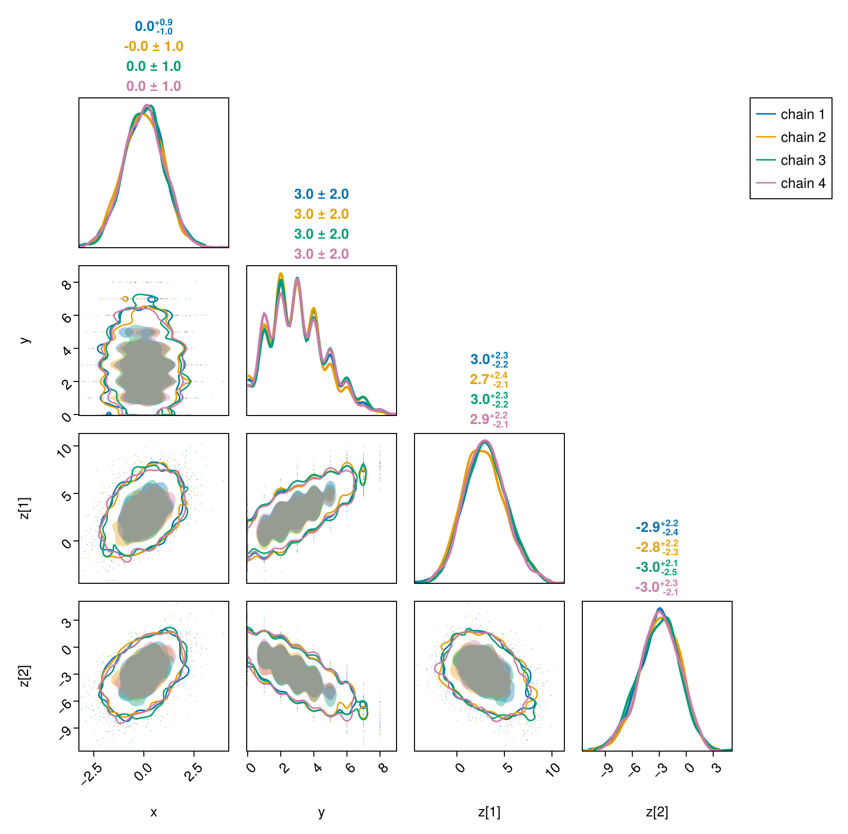
Many visualisation functions with both Makie.jl and Plots.jl backends are provided, along with a PairPlots.jl extension.
using PairPlots, CairoMakie
pairplot(chain)